Tutorial

The package contains two classes xmca.array.MCA for numpy.ndarray and xmca.xarray.xMCA for xarray.DataArray. Depending on which data type you work with, import the respective module:

from xmca.array import MCA  # numpy
from xmca.xarray import xMCA  # xarray

For this tutorial we use North American surface temperatures from 2013 to 2014 shipped with xarray. We arbitrarily separate the data into two domains, west and east.

import xarray as xr  # only needed to obtain test data

# split data arbitrarily into west and east coast
data = xr.tutorial.open_dataset('air_temperature').air
west = data.sel(lon=slice(200, 260))
east = data.sel(lon=slice(260, 360))

Note

xMCA only accepts DataArray, not Dataset.

Warning

The time coordinate needs to be called time, the spatial coordinates lat and lon. In particular ERA5 data sets have their spatial coordinates labeled as longitude and latitude. Consider renaming via e.g. era5 = era5.rename({'longitude':'lon', 'latitude':'lat'}).

PCA/MCA

Performing standard MCA is straightforward. Simply run:

mca = xMCA(west, east)
mca.solve()

The singular values (= eigenvalues), spatial patterns (EOFs) and the expansion coefficients (PCs) can then be obtained via

svals = mca.singular_values()
expvar = mca.explained_variance()

eofs  = mca.eofs()
pcs   = mca.pcs()

Note

To perform PCA/EOF analysis instead of MCA, simply provide one instead of two fields, e.g. pca = xMCA(west).

Retrieve the homogeneous and heterogeneous patterns through

hom_patterns = mca.homogeneous_patterns()
het_patterns  = mca.heterogeneous_patterns()

Note

All methods that provide quantities for both left and right field (pcs, eofs etc.) return dictionaries with keys left and right for the respective field. If PCA is performed, only left exists.

Pre-processing

By calling the constructor, the input fields are centered (mean removed). Additionally, by using normalize the input fields are standardized. In order to weight the input fields according to their area on a sphere, that is each grid point is multiplied by \(\sqrt{ \cos (\varphi_i)}\) with \(\varphi\) being the latitude, apply_coslat can be used.

mca = xMCA(west, east)
mca.normalize()
mca.apply_coslat()
mca.solve()

Warning

Always call apply_coslat after normalize since the latter nullifies the latitude weighting.

Rotated MCA

The package provides two rotation schemes:

1. Varimax orthogonal rotation [1] and

2. Promax oblique rotation [2]

Both are available through rotate where specifying the number of rotated EOFs (n_rot) and the Promax parameter (power) defines the type of rotation. For example, to perform Varimax-rotated MCA on the first 10 EOFs run:

mca = xMCA(west, east)
mca.solve()
mca.rotate(n_rot=10, power=1)

Now retrieving the rotated PCs/EOFs works the same as before for standard MCA. Note that the singular values are not affected by the rotation. If you want to obtain the (co-)variance associated to each mode, use the variance method, which is also used to determine the explained variance after rotation.

svals = mca.singular_values()  # same as before rotation
variance = mca.variance()  # different from singular values
rotated_expvar = mca.explained_variance()  # different after rotation

rotated_eofs  = mca.eofs()
rotated_pcs   = mca.pcs()

If for some reason you want to obtain the unrotated PCs/EOFs after the model has been rotated, the rotated parameter comes in handy.

unrotated_eofs  = mca.eofs(rotated=False)
unrotated_pcs   = mca.pcs(rotated=False)

Note

For standard MCA, the results of singular_values and variance are identical. In fact, for standard MCA each singular value is indeed just the covariance explained by the respective mode.

Complex MCA

Complex PCA/MCA [3, 4] provides a means to investigate lagged correlations and spatially moving patterns. Performing complex MCA is similarly straightforward:

mca = xMCA(west, east)
mca.solve(complexify=True)

However, when the input data is not stationary, spectral leakage inherent to the Hilbert transform can sometimes produce strong boundary effects which affect the obtained PCs. One approach to mitigate these effects is by artificially extending the input time series before the Hilbert transform and then truncating it afterwards. Here, two different extension methods are provided:

1. Theta model extension [5] (èxtend='theta')

2. Exponential decay superimposed on a linear trend (èxtend='exp')

Both approaches require an additional parameter ``period```which has to be chosen a priori.

As a result of complex MCA, the EOFs and PCs have a real and imaginary part. This allows to compute the spatial amplitude and phase function as well as the temporal amplitude and phase function:

s_amp = mca.spatial_amplitude()
s_phase = mca.spatial_phase()
t_amp = mca.temporal_amplitude()
t_phase = mca.temporal_phase()

Note

By combining solve(complexify=True) and rotate, one can perform complex rotated PCA/MCA.

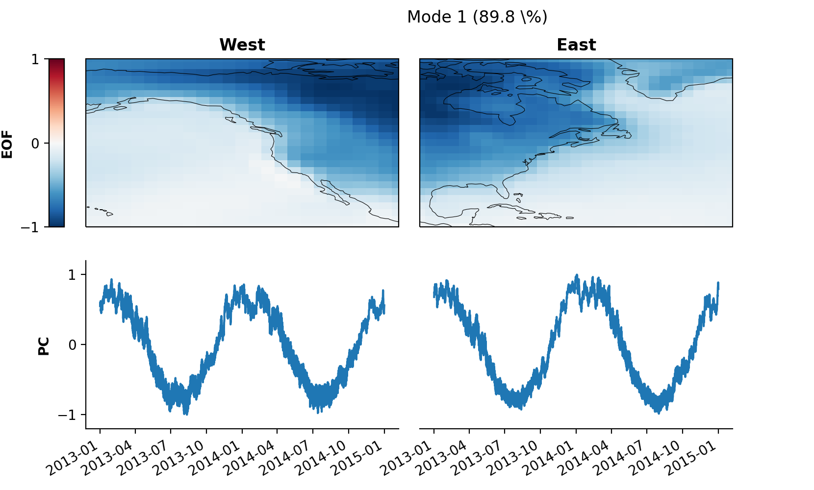
Visualization

The package provides a plot method to visually inspect the individual modes.

mca.set_field_names('West', 'East')
pkwargs = {'orientation' : 'vertical'}
mca.plot(mode=1, **pkwargs)

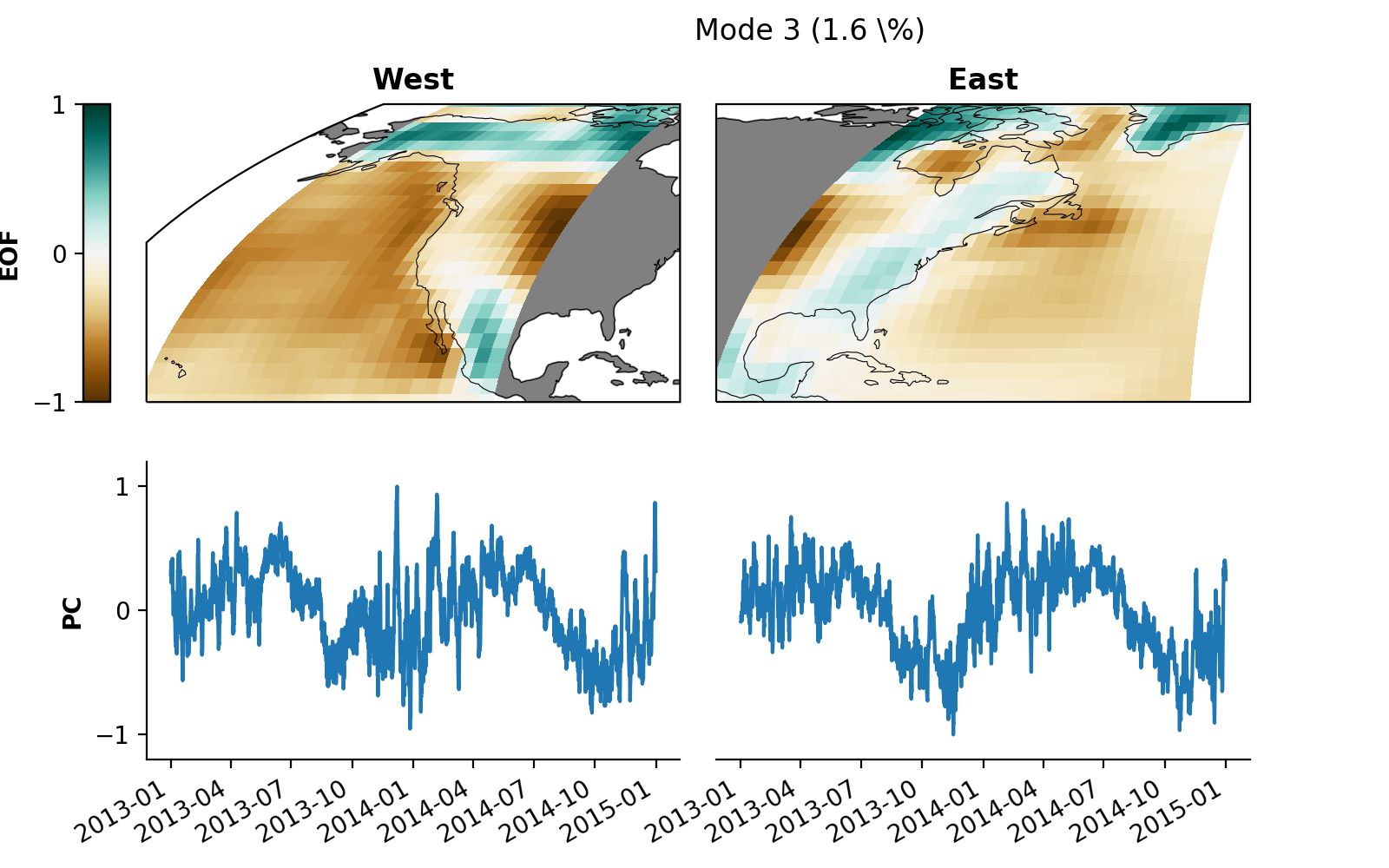
Some fine-tuning of the plot for better optics:

from cartopy.crs import EqualEarth  # for different map projections

# map projections for "left" and "right" field
projections = {
    'left': EqualEarth(),
    'right': EqualEarth()
}

pkwargs = {
    "figsize"     : (8, 5),
    "orientation" : 'vertical',
    'cmap_eof'    : 'BrBG',  # colormap amplitude
    "projection"  : projections,
}
mca.plot(mode=3, **pkwargs)

You can save the plot to your local disk as a .png file via

skwargs={'dpi':200, 'transparent':True}
mca2.save_plot(mode=3, plot_kwargs=pkwargs, save_kwargs=skwargs)

Evaluation

xmca provides some methods to assess the significance of the obtained modes:

1. North’s rule of thumb

2. Rule N

3. Bootstrapping

North’s Rule of Thumb

We can obtain the error estimates of the singular values via rule_north.

svals_err_north = mca.rule_north().to_dataframe()
svals_diff = svals.to_dataframe().diff(-1)
cutoff = np.argmax((svals_diff - (2 * svals_err_north)) < 0)  # 10

According to North’s Rule of Thumb [6], mode 10 is the first “effective multiplet”, that is given the sample size it cannot be resolved from the neighboring singular value.

Rule N

The aim of Rule N [7] is to provide a rule of thumb for the significance of the obtained singular values via Monte Carlo simulations of uncorrelated Gaussian random variables. The obtained singular values are scaled such that their sum equals the sum of true singular value spectrum. Under these assumptions we can use rule_n choosing the number of Monte Carlo simulations.

svals_rule_n = mca.rule_n(n_runs=100)
median = svals_rule_n.median('run')
q99 = svals_rule_n.quantile(.99, dim='run')
cutoff = np.argmax((svals < q99).values)  # 10

Here we defined the cutoff as the mode where the 99th quantile of the Rule N distribution exceeds the sampled singular value. In this case the cutoff according to Rule N is at mode 10.

Bootstrapping

bootstrapping provides a flexible method to perform a wide range of different Monte Carlo simulations. By specifying axis, samples are either drawn along time (0) or along space (1). The parameters on_left and on_right specify which field should be re-sampled. When both are True, samples are drawn from the joint distribution of both fields. For serially correlated variables, the block_size parameter provides the possibility to run moving-block bootstraps by re-sampling blocks of data. By default, re-sampling is performed with replacement. This can be turned off, however, by choosing replace=False which basically means permutation.

Here we perform bootstrapping (with replacement) along space of the joint distribution in order to assess the confidence interval of the singular values. This procedure suggest that the first 4 modes are significant.

svals_boot = mca.bootstrapping(100, on_left=True, on_right=True, axis=1, replace=False)
boot_q01 = svals_boot.quantile(0.01, 'run')
boot_q99 = svals_boot.quantile(0.99, 'run').shift({'mode' : -1})
cutoff = np.argmax((boot_q01 - boot_q99).dropna('mode').values < 0)  # 4

Note

You usually want to run large numbers of Monte Carlo simulations. A typical rule of thumb is \(40N\) where N is the number of observations (time steps) in your input data.

Saving an analysis

It is possible to save and load the model via save_analysis in a provided path. A info file info.xmca is then created in this directory which can be loaded via load_analysis.

mca.save_analysis('my_analysis')

new = xMCA()
new.load_analysis('my_analysis/info.xmca')

Warning

The original input fields are saved along with the singular vectors, allowing to call pcs, heterogeneous_patterns etc. However, evaluation results are not saved, in particular no bootstrap results.

1

Kaiser, H. F. The varimax criterion for analytic rotation in factor analysis. Psychometrika 23, 187–200 (1958).

2

Hendrickson, A. E. & White, P. O. Promax: A Quick Method for Rotation to Oblique Simple Structure. British Journal of Statistical Psychology 17, 65–70 (1964).

3

Horel, J. Complex Principal Component Analysis: Theory and Examples. J. Climate Appl. Meteor. 23, 1660–1673 (1984).

4

Rieger, N., Corral, Á., Olmedo, E. & Turiel, A. Lagged teleconnections of climate variables identified via complex rotated Maximum Covariance Analysis. submitted (2021).

5

Assimakopoulos, V. & Nikolopoulos, K. The theta model: a decomposition approach to forecasting. International Journal of Forecasting 16, 521–530 (2000).

6

North, G., L. Bell, T., Cahalan, R. & J. Moeng, F. Sampling Errors in the Estimation of Empirical Orthogonal Functions. Monthly Weather Review 110, (1982).

7

Overland, J.E., Preisendorfer, R.W., 1982. A significance test for principal components applied to a cyclone climatology. Mon. Weather Rev. 110, 1–4.

8

Efron, B., Tibshirani, R.J., 1993. An Introduction to the Bootstrap. Chapman and Hall. 436 pp.