Quickstart¶

Import the module for xarray via

from xmca.xarray import xMCA

As an example, we take North American surface temperatures shipped with xarray. Note: only works with``xr.DataArray``, not ``xr.Dataset``.

import xarray as xr  # only needed to obtain test data

# split data arbitrarily into west and east coast
data = xr.tutorial.open_dataset('air_temperature').air
west = data.sel(lon=slice(200, 260))
east = data.sel(lon=slice(260, 360))

Principal Component Analysis¶

pca = xMCA(west)                    # PCA of west coast
pca.solve(complexfify=False)        # True for complex PCA
#pca.rotate(10)                     # optional; Varimax rotated solution
                                    # using 10 first EOFs
eigenvalues = pca.singular_values() # singular vales = eigenvalues for PCA
pcs         = pca.pcs()             # Principal component scores (PCs)
eofs        = pca.eofs()            # spatial patterns (EOFs)

Maximum Covariance Analysis¶

mca = xMCA(west, east)                     # MCA of field A and B
mca.solve(complexfify=False)        # True for complex MCA
#mca.rotate(10)                     # optional; Varimax rotated solution
                                    # using 10 first EOFs
eigenvalues = mca.singular_values() # singular vales
pcs = mca.pcs()                     # expansion coefficient (PCs)
eofs = mca.eofs()                   # spatial patterns (EOFs)

Save/load an analysis¶

mca.save_analysis('my_analysis')    # this will save the data and a respective
                                    # info file. The files will be stored in a
                                    # special directory
mca2 = xMCA()                       # create a new, empty instance
mca2.load_analysis('my_analysis/info.xmca') # analysis can be
                                    # loaded via specifying the path to the
                                    # info file created earlier

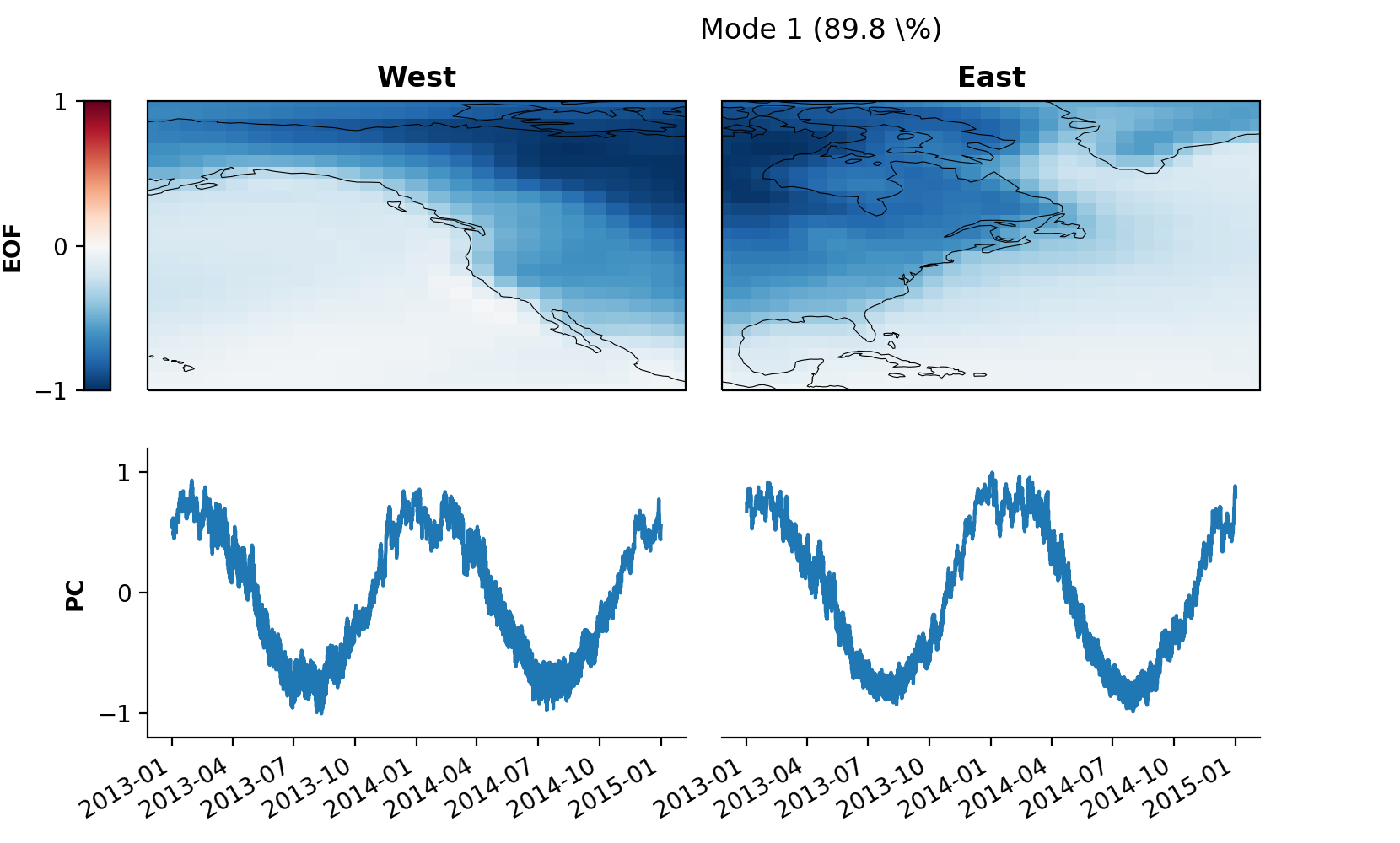
Plot your results¶

The package provides a method to visually inspect the individual modes.

mca2.set_field_names('West', 'East')
pkwargs = {'orientation' : 'vertical'}
mca2.plot(mode=1, **pkwargs)

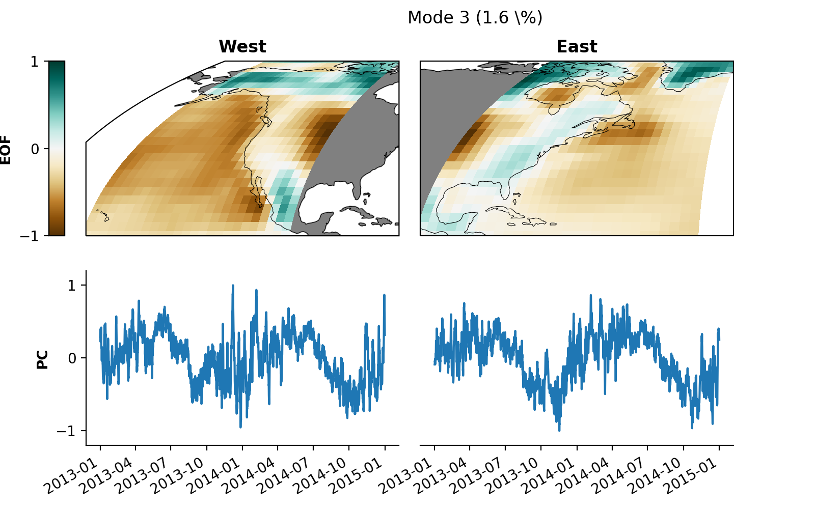
Result of default plot method after performing MCA on T2m of North American west and east coast showing mode 1.

You may want to modify the plot for some better optics:

from cartopy.crs import EqualEarth  # for different map projections

# map projections for "left" and "right" field
projections = {
    'left': EqualEarth(),
    'right': EqualEarth()
}

pkwargs = {
    "figsize"     : (8, 5),
    "orientation" : 'vertical',
    'cmap_eof'    : 'BrBG',  # colormap amplitude
    "projection"  : projections,
}
mca2.plot(mode=3, **pkwargs)

Result of plot method with improved optics after performing MCA on T2mof North American west and east coast showing mode 3.

You can save the plot to your local disk as a .png file via

skwargs={'dpi':200, 'transparent':True}
mca2.save_plot(mode=3, plot_kwargs=pkwargs, save_kwargs=skwargs)